Assigning volunteers to work areas
Explore these skills in a real word context.
A sample space lists of all the possible outcomes, giving a complete picture of the situation. Sample spaces form the foundation for calculating probabilities and making predictions about future events. Use this resource to learn some ways to represent a sample space.
A sample space is a list or diagram showing all possible outcomes in a probability experiment.
We can rewrite the probability equation to:
\[\begin{align*} \Pr(E) & = \frac{\textrm{Number of ways $E$ can occur}}{\textrm{Number of outcomes in the sample space}}\\
& = \frac{n(E)}{n(S)}
\end{align*}\]
Again, this assumes all outcomes are equally likely.
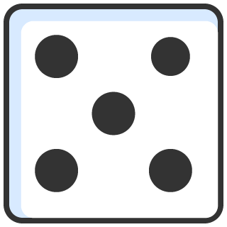
For tossing a single die, the sample space is \(1,2,3,4,5,6\). We can immediately tell that \(\Pr(1)=\Pr(2)=\Pr(3)=\Pr(4)=\Pr(5)=\Pr(6)=\dfrac{1}{6}\).
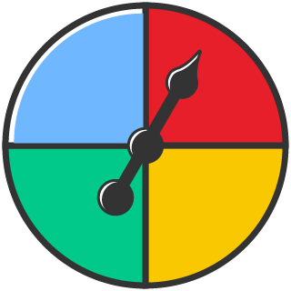
For a four-colour spinner with equal sectors, the sample space is Red, Green, Yellow, Blue. \(\Pr(R)=\Pr(G)=\Pr(Y)=\Pr(B)=\dfrac{1}{4}\).
The sum of the probabilities of the distinct outcomes within a sample space is \(1\).
Let's look into some ways to represent sample spaces.
A tree diagram can be used to find the sample space. It uses a branching format, starting from a single point and splitting into paths that represent different possibilities. Each branch represents an event and the complete diagram shows all outcomes at the ends of the branches.
Use a tree diagram to find the sample space for two coins tosses, then determine the probability of getting at least one head.
There are two possible outcomes for each toss: H = Heads and T = Tails. We draw one branch to represent the outcomes of the first coin toss: H or T. Then, from each of these initial outcomes, we draw another branch: H or T.
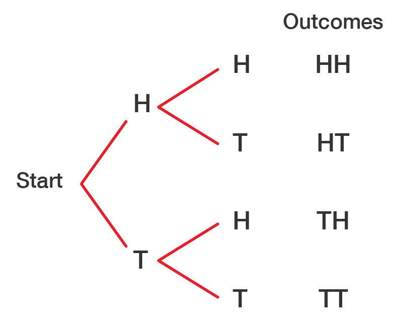
The image is a tree diagram showing all possible outcomes for two consecutive coin flips, starting from the "Start" point.
The sample space for tossing the two coins is: HH HT TH TT. We can see that each has a probability of \(\dfrac{1}{4}\).
To find the probability of at least one head, we need to add up the probabilities of getting HH, HT or TH:
\[\begin{align*} \Pr(HH\cup HT\cup TH) & = \frac{1}{4}+\frac{1}{4}+\frac{1}{4}\\
& = \frac{3}{4}
\end{align*}\]
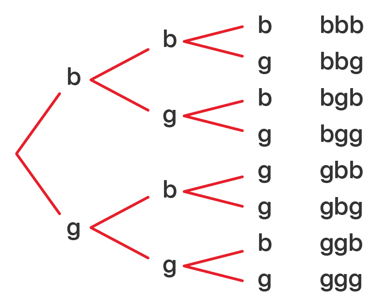
Let's let b = boy and g = girl. There are two possible outcomes for each child: b or g. There are three children, so we need three branches.
The image is a tree diagram showing all possible outcomes for a family with three children.
The sample space for a three child family is: bbb, bbg, bgb, bgg, gbb, gbg, ggb, ggg.
To find the probability of the first child being a girl, we need to add up the probabilities of getting gbb, gbg, ggb or ggg. Each has a \(\dfrac{1}{8}\) possibility of occurring.
\[\begin{align*} \Pr(ggb\cup gbg\cup ggb\cup ggg) & = \frac{1}{8}+\frac{1}{8}+\frac{1}{8}+\frac{1}{8}\\
& = \frac{4}{8}\\
& = \frac{1}{2}
\end{align*}\]
Tables are helpful to organise information that makes finding probabilities easier. Let's see an example.
The following table shows the results of a study that looked at the association between smoking (S) and lung cancer (C).
| Lung cancer | No lung cancer | Total | |
|---|---|---|---|
| Smoker | \(30\) | \(70\) | \(100\) |
| Non-smoker | \(10\) | \(90\) | \(100\) |
| \(40\) | \(160\) | \(200\) |
Find the probability that an individual:
There are \(100\) smokers out of the total \(200\) individuals, so:
\[\begin{align*} \Pr(S) & = \frac{100}{200}\\
& = \frac{1}{2}
\end{align*}\]
There are \(160\) individuals of the \(200\) who do not have lung cancer, so:
\[\begin{align*} \Pr(C') & = \frac{160}{200}\\
& = \frac{4}{5}
\end{align*}\]
There are \(30\) individuals of the \(200\) who are smokers and have lung cancer, so:
\[\begin{align*} \Pr(S\cap C) & = \frac{30}{200}\\
& = \frac{3}{20}
\end{align*}\]
Venn diagrams are also handy for showing sample spaces. They consist of overlapping circles to show relationships between different sets of outcomes in a probability experiment.
Each circle shows a group of outcomes. They overlap where outcomes are common to those groups.
Venn diagrams are especially useful for showing how events relate to each other, such as mutually exclusive events.
The Venn diagram shows the number of people in a survey who regularly ate KitKats (K), Mars bars (M) or Rocky Road (R).
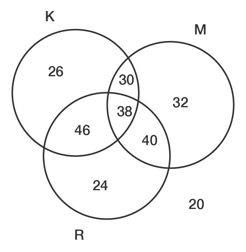
From the Venn diagram, we can see that there are \(256\) people. This is the sum of all sections of the diagram: \(26+46+30+38+40+24+32+20\).
People who eat KitKats include those who:
This is \(26+30+46+38=140\) of the \(256\) people, so:
\[\begin{align*} \Pr(K) & = \frac{140}{256}\\
& = \frac{35}{64}
\end{align*}\]
There are \(40\) people who eat Mars bars and Rocky Road, but also \(38\) people who eat all three, so:
\[\begin{align*} \Pr(M\cap R) & = \frac{40+38}{256}\\
& = \frac{78}{256}\\
& = \frac{39}{128}
\end{align*}\]
There are \(30\) people who eat KitKats and Mars bars, but not Rocky Road, so:
\[\begin{align*} \Pr(K\cap M\cap R') & = \frac{30}{256}\\
& = \frac{15}{128}
\end{align*}\]
There are \(20\) people who do not eat any of these, so the rest of the people must eat at least one. Therefore:
\[\begin{align*} \Pr(K\cup M\cup R) & = 1-\Pr(K\cup M\cup R)'\\
& = 1-\frac{20}{256}\\
& = \frac{236}{256}\\
& = \frac{59}{64}
\end{align*}\]
This is the same as adding up all the numbers inside the Venn diagram:
\[\begin{align*} \Pr(K\cup M\cup R) & \frac{26+46+38+30+32+40+24}{256}\\
& = \frac{236}{256}\\
& = \frac{59}{64}
\end{align*}\]
Depending on the type of data, it may help to use a unique diagram to represent the sample space.
The sample space for a deck of \(52\) cards is shown. Find the probability of the event (E) where the card drawn is a diamond (D) or an ace (A).
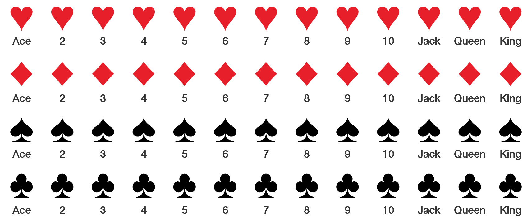
\(\dfrac{1}{4}\) of the cards are diamonds. \(\dfrac{4}{52}\) are aces. Therefore:
\[\begin{align*} \Pr(E) & = \Pr(D\cup A)\\
& = \Pr(D)+\Pr(A)-\Pr(D\cap A)\\
& = \frac{13}{52}+\frac{4}{52}-\frac{1}{52}\\
& = \frac{16}{52}\\
& = \frac{4}{13}
\end{align*}\]
| \(\mathbf{1}\) | \(\mathbf{2}\) | \(\mathbf{3}\) | \(\mathbf{4}\) | \(\mathbf{5}\) | \(\mathbf{6}\) | |
|---|---|---|---|---|---|---|
| \(\mathbf{1}\) | \((1,1)\) | \((1,2)\) | \((1,3)\) | \((1,4)\) | \((1,5)\) | \((1,6)\) |
| \(\mathbf{2}\) | \((2,1)\) | \((2,2)\) | \((2,3)\) | \((2,4)\) | \((2,5)\) | \((2,6)\) |
| \(\mathbf{3}\) | \((3,1)\) | \((3,2)\) | \((3,3)\) | \((3,4)\) | \((3,5)\) | \((3,6)\) |
| \(\mathbf{4}\) | \((4,1)\) | \((4,2)\) | \((4,3)\) | \((4,4)\) | \((4,5)\) | \((4,6)\) |
| \(\mathbf{5}\) | \((5,1)\) | \((5,2)\) | \((5,3)\) | \((5,4)\) | \((5,5)\) | \((5,6)\) |
| \(\mathbf{6}\) | \((6,1)\) | \((6,2)\) | \((6,3)\) | \((6,4)\) | \((6,5)\) | \((6,6)\) |
Find the probability that:
Images on this page by RMIT, licensed under CC BY-NC 4.0

RMIT University acknowledges the people of the Woi wurrung and Boon wurrung language groups of the eastern Kulin Nation on whose unceded lands we conduct the business of the University. RMIT University respectfully acknowledges their Ancestors and Elders, past and present. RMIT also acknowledges the Traditional Custodians and their Ancestors of the lands and waters across Australia where we conduct our business - Artwork 'Sentient' by Hollie Johnson, Gunaikurnai and Monero Ngarigo.
More information