Poisson distribution

The Poisson distribution deals with the number of random occurrences over a period of time or a given space, such as the number of people who enter a shop every hour or the number of flaws in a sheet of glass. It is very handy, well beyond applications in STEM. Use this resource to learn how to use the Poisson distribution.

The Poisson distribution is a discrete distribution like the binomial distribution. This means that it involves events that we can count. It measures the probability that a certain number of random independent events occur within a period of time (or distance or area, etc.) when the average rate of occurrence is known.

It was developed in the \(1800\)s when mathematicians were asked to theorise on such matters as the annual number of wrongful criminal convictions in a particular country or to work out the number of soldiers in the Prussian cavalry who were likely to be kicked to death by a horse (honest!)

Some more modern examples of events described by a Poisson distribution distribution are:

• the number of errors or crashes a software system experiences in a day
• number of online orders received for a particular item per hour during a sale
• the numbers of cars that pass on a stretch of road over a certain time period
• the number of stars in a given area of a telescope's field of view
• the number of communication failures within a specific network area
• the number of phone calls a customer support centre receives per minute.

Poisson probabilities

Poisson probabilities are calculated using:

\[\Pr(X=x)=\frac{e^{-\lambda}\lambda^{x}}{x!}\]

where \(\lambda\) is the mean or expected number of occurrences per unit of time, distance, area or volume.

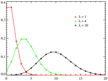
The Poisson distribution varies with \(\lambda\).

• As \(\lambda\) increases, the shape of the Poisson distribution becomes more spread out and symmetric. The average rate of occurences is higher, so the distribution looks more like a normal distribution.
• For smaller \(\lambda\) values, most probabilities cluster around \(x=0\). In other words, when the average rate of occurence is small, the likelihood of observing a higher number of events is very small.

Example – calculating Poisson probabilities

Suppose that over the past years, a company receives an average of \(3\) defective returns from customers each month. What is the probability that next month there will be \(4\) defective returns?

Here, \(\lambda=3\) as it is the average or expected value. The number of successes is \(x=4\). We can use these values to calculate the probability.
\[\begin{align*} \Pr(X=x) & = \frac{e^{-\lambda}\lambda^{x}}{x!}\\
& = \frac{e^{-3}3^{4}}{4!}\\
& = \frac{81e^{-3}}{4\times3\times2\times1}\\
& = 0.168
\end{align*}\]

Approximating the binomial distribution

Often, the normal distribution can be used to get fairly good approximations of binomial probabilities. This works best when \(p\) is close to \(0.5\). The normal distribution becomes closer to the binomial probability as \(n\) increases.

As a general rule, both \(np\) and \(n(1-p)\) should be greater than or equal to \(5\) in order to use the normal approximation.

But, what if these rules are not satisfied? If \(p<0.05\) and \(n\) is large, we can use the Poisson distribution to approximate the binomial distribution. When we do this, we calculate \(\lambda\):

\[\lambda=np\]

Example – approximating binomial distributions

A sample of \(50\) plants are taken from a field, where \(1\%\) of the plants are expected to have a certain pest infection. What is the probability that \(2\) of these plants are infested? Compare the binomial probability and the probability approximated using the Poisson distribution.

Using the binomial distribution, we have \(n=50\), \(p=0.01\) and \(1-p=0.99\). To calculate the probability for a binomially distributed data, we use \(\Pr(X=x)=^{n}C_{x}\times p^{x}\times(1-p)^{n-x}\).
\[\begin{align*} ^{n}C_{x} & = \frac{n!}{x!(n-x)!}\\
& = \frac{50!}{2!(50-2)!}\\
& = 1225
\end{align*}\] \[\begin{align*} \Pr(X=2) & = ^{n}C_{x}\times p^{x}\times(1-p)^{n-x}\\
& = ^{50}C_{2}\times p^{2}\times(1-50)^{50-2}\\
& = 1225\times0.01^{2}\times0.99^{48}\\
& = 0.0756
\end{align*}\]

To approximate the binomial probability using the Poisson distribution, we first need to calculate \(\lambda\).
\[\begin{align*} \lambda & = np\\
& = 50\times0.01\\
& = 0.5
\end{align*}\]

Then, we can use the Poisson approximation equation.

\[\begin{align*} \Pr(X=2) & = \frac{e^{-\lambda}\lambda^{x}}{x!}\\
& = \frac{e^{-0.5}0.5^{2}}{2!}\\
& = 0.0758
\end{align*}\]

The binomial probability is \(0.0756\) and the approximation is \(0.0758\). You can see that the Poisson distribution gives a good approximation. It would be even more accurate if \(n\) was larger.

Exercise – approximating binomial distributions

1. On average, one in every \(100\) births produces twins. Use the Poisson distribution to find the probability that there is one set of twins in the next \(250\) births.
2. A manufacturer of electric light globes knows from past experience that \(2\%\) of globes produced are defective. Use the Poisson distribution to approximate the probability that, out of the next \(200\) globes, less than \(2\) are defective?
3. The chance of death by drowning is \(\dfrac{1}{30000}\). Use the Poisson distribution to estimate the probability that, out of a random selection of \(1500\) people, there will be at least one death by drowning.
4. Insurance companies have found that the probability that a residential property is damaged by fire at some stage over a \(25\) year period is \(0.01\). If a company insures \(20\) homes in a particular street, use the Poisson distribution to approximate the probability that \(2\) of them will be damaged by fire in the next \(25\) years.