Rather than comparing a sample mean to a population mean, we can compare a sample proportion to a population proportion. These tests of proportion are used broadly, like for checking if a new fabric meets quality standards by having fewer defects or evaluating customer satisfaction levels for financial services. Use this resource to learn how to perform tests of proportions.
A test of proportion is used to determine whether or not a sample from a population represents the true proportion from the entire population.
Tests of proportion are useful when we want to compare categorical data, like the percentage of defective items in a batch or the proportion of people preferring a new product over an old one. They help organisations make informed decisions based on sample data.
Conducting tests of proportions
Again, the process of conducting a test of proportions is similar to what you have already encountered for \(z\)- and t-tests.
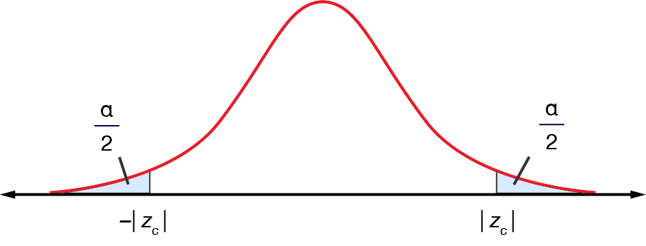
State the null and alternative hypotheses. We can let \(\hat{p}\) (or \(\pi\)) be the sample proportion and \(p\) be the null hypothesised population proportion. For a two-tailed test:
\(H_{0}:\hat{p}=p\) (the proportion of the population from which the sample is drawn is the same as the given population proportion)
\(H_{a}:\hat{p}\neq p\) (the proportion of the population from which the sample is drawn is not the same as the given population proportion)
Choose a significance level. Often, we choose \(\alpha=0.05\).
Find the critical values \(z_{c}\) using a \(z\)-table.
If \(np>5\) and \(n(1-p)>5\), we assume that the test statistic is normally distributed. If these are not satisfied, we should make note of this, or use a different and more exact test.
Calculate the test statistic.
\[z = \frac{ \hat{p}-p}{\sqrt{\frac{p(1-p)}{n}}}\]
Compare the test statistic to the critical value to make a decision about the null hypothesis. If the test statistic is more extreme than the critical value, we reject the null hypothesis. If not, we do not reject the null hypothesis.
Draw a conclusion from the hypothesis test.
If we have rejected the null hypothesis, this means that the proportion of the population from which the sample is drawn is not the same as the given population proportion after allowing for chance variation.
If we have not rejected the null hypothesis, this means that the proportion of the population from which the sample is drawn is the same as the given population proportion after allowing for chance variation.
Example – conducting tests of proportion
A lecturer knows that, historically, \(60\%\) of students do not begin their statistics assignment until within seven days of the due date. As a result, they do not do well. To address this unfortunate reality, Maths support services are widely promoted during the early weeks of the semester.
A survey of \(80\) randomly selected students revealed that \(42\) had started the assignment before the final week. Is there evidence to suggest the promotion had been effective at the \(10\%\) significance level?
In this case, \(\hat{p}=\dfrac{42}{80}=0.525\). The hypotheses would be:
\(H_{0}:\hat{p}=0.6\)
\(H_{a}:\hat{p}<0.6\)
The significance level has already been set for us at \(\alpha=0.10\).
To make sure that the test statistic is normally distribution, we need to check that \(np>5\) and \(n(1-p)>5\).
\(np=48\)
\(n(1-p)=32\)
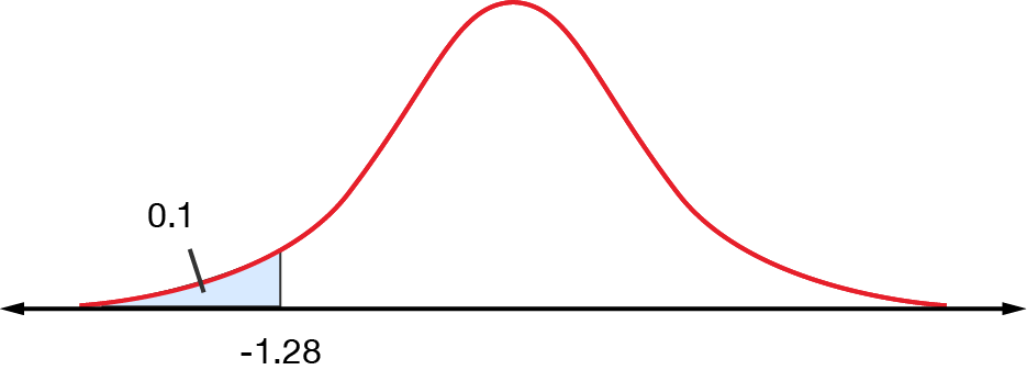
It is normally distributed, so we can use the \(z\)-table to find the critical value, \(z=-1.28\).
We then find the test statistic.
\[\begin{align*} z & = \frac{ \hat{p}-p}{\sqrt{\frac{p(1-p)}{n}}}\\
& = \frac{0.525-0.6}{\sqrt{\frac{0.6(1-0.6)}{80}}}\\
& = -1.37
\end{align*}\]
\(-1.37\) is more extreme than \(-1.28\); therefore, we reject the null hypothesis.
There is evidence to suggest that the promotion has been effective and that students are beginning their assignments earlier.
Exercises – conducting tests of proportion
A survey conducted in \(2012\) showed that \(18\%\) of students were the first in their family to attend university. To evaluate widening participation programs, a randomly selected sample of \(120\) enrolment records indicated that in \(2017\), this number had increased to \(24\%\). Does this data provide convincing evidence to suggest that the percentage of "first in family" students has changed over these five years? Use \(\alpha=0.10\).
A car manufacturer advertises that at least \(80\%\) of vehicles will obtain fuel economy of \(7\textrm{ L}/100\textrm{ km}\) or better. To test the claim, a consumer interest group randomly selects \(22\) vehicles and finds that only \(15\) achieve this figure. Is there evidence that the company's claim is false at the \(5\%\) level of significance?
In a rural community hospital, \(6\) out of \(7\) babies born in a particular week were boys. Assuming that in the general population, the probability of female and male babies is equal, test the claim that babies born at this hospital are more likely to be boys at the \(10\%\) level of significance.
\(z=1.71\) so we reject the null hypothesis. There is enough evidence to suggest that the percentage of "first in family" students has changed between \(2012\) and \(2017\).
\(z=-1.41\) so we do not reject the null hypothesis. There is not enough evidence to suggest that the company's claim is false.
\(z=1.89\) so we reject the null hypothesis but note that the data does not appear to be normally distributed. We could say that there is enough evidence to suggest that babies born at the hospital are more likely to be boys, but the claim might not be reliable.
Unless otherwise labelled, images on this page by RMIT, licensed under CC BY-NC 4.0