T-tests

T-tests help us understand if the differences we observe in data are due to random chance or if they're meaningful. They are commonly used in research to compare groups, like testing if a new teaching method improves scores more than the old one. Use this resource to learn how to use t-tests to test hypotheses.

T-distribution

Hypothesis testing usually uses the population standard deviation (\(\sigma\)) to calculate a \(z\)-score. If the population standard deviation is unknown, we approximate using the sample standard deviation (\(s\)):

\[s_{\overline{x}}=\frac{s}{\sqrt{n}}\]

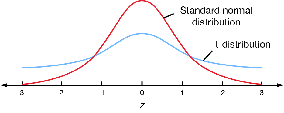
A sampling distribution that results from approximating \(\sigma\) with \(s\) is called a t-distribution. The t-distribution curve is a bit distorted compared to the standard normal distribution. This is because \(\sigma\) is a fixed value and \(s\) varies with each sample. The varied \(s\) creates a level of uncertainty.

The precise shape of the t-distribution depends on the size of the sample. It is always bell-shaped but varies slightly according to the size of the sample \(n\). As the sample size increases, a t-distribution becomes more like the standard normal distribution distribution. For small \(n\) values, it has heavier tails.

T-tests

Like the \(z\)-test, a t-test is a hypothesis test used to make decisions about the similarity of sample and population means.

It involves calculating a test statistic called the t-value:
\[t = \frac{\overline{x}-\mu}{\frac{s}{\sqrt{n}}} \]

You might notice that the equation is almost identical to the test statistic for a \(z\)-test, but \(s\) is used instead of \(\sigma\).

Like a \(z\)-test, we assume that the sample data is drawn randomly and that the distribution of sample means follows a normal distribution.

Conducting t-tests

The process for conducting a t-test is similar to that for a \(z\)-test, but using an additional parameter and a \(t\)-table.

1. State the null and alternate hypotheses.
• \(H_{0}:\overline{x}=\mu\) (the sample mean is the same as the population mean after allowing for chance variation)
• \(H_{a}:\overline{x}\neq\mu\) (the sample mean is not the same as the population mean after allowing for chance variation)
2. Choose a significance level. Often, we choose \(\alpha=0.05\). In other words, we define "reasonable" as what we can expect \(95\%\) of the time.
3. Find the critical values (\(t_{c}\)) that correspond to the chosen significance level, \(\alpha\). Te critical t-value also depends on the degrees of freedom, \(n-1\). This is the number of separate pieces of information that we need to calculate a statistic.

   These \(t\)-values are the cutoff points beyond which we reject the null hypothesis.

4. Calculate the test statistic. This is the standardised difference between the sample mean (calculated from the data) and the known population mean:
   \[t = \frac{\overline{x}-\mu}{\frac{s}{\sqrt{n}}}\]
5. Compare the test statistic to the critical value to make a decision about the null hypothesis.
• If the test statistic falls beyond the cutoff point/s of the critical value, we reject the null hypothesis with \(5\%\) confidence, as per the chosen significance level.
• If the test statistic falls within the cuttoff point/s of the critical value, we do not reject the null hypothesis with \(5\%\) confidence, as per the chosen significance level.
6. Draw a conclusion from the hypothesis test.
• If we have rejected the null hypothesis, this means that the sample mean is not the same as the population mean after allowing for chance variation.
• If we have not rejected the null hypothesis, this means that the sample mean is the same as the population mean after allowing for chance variation.

Just like for \(z\)-tests, remember:

• The decision about the null hypothesis is not made with certainty but with a level of confidence that the error in the decision is small; for example, \(5\%\) if \(\alpha=0.05\).
• Terminology is important! The decision relates only to rejecting or not rejecting the null hypothesis, \(H_{0}\). We never make a decision that references the alternate hypothesis, \(H_{a}\), nor do we say we "accept" either hypothesis.

T-test or \(z\)-test?

Sometimes, it can be confusing whether to use a \(z\)-test or a t-test to test your hypothesis.

Generally:

• use a \(z\)-test if you know \(\sigma\)
• use a t-test if you do not know \(\sigma\).

But there may be some exceptions!

• Many textbooks only provide t-tables for \(n\leq30\). For larger samples, the standard normal distribution is a reasonable approximation and a \(z\)-test may be used even though \(\sigma\) is unknown.
• Some courses provide students with more comprehensive t-tables for \(n\) up to \(50\) or \(100\). If you have access to such tables, you should use a t-test whenever \(\sigma\) is not known, no matter the size of the sample.
• If you know that \(s\) is a good approximation for \(\sigma\), then a \(z\)-test may be appropriate.
• If a computer package such as SPSS, Minitab or Microsoft Excel is being used for the hypothesis test, then a t-test should be selected when \(\sigma\) is unknown.

Example – conducting t-tests

A manufacturer of batteries claims that, on average, a battery lasts \(200\) hours. To test this claim, \(7\) batteries were randomly selected and the sample had an average of only \(190\) hours with a standard deviation of \(9\) hours. Does this sample provide evidence at the \(1\)% level of significance that the manufacturers claim is incorrect?

1. We start with the hypotheses.
   • \(H_{0}:\mu_{\overline{x}}=200\)
   • \(H_{a}:\mu_{\overline{x}}\neq200\)
2. The significance level has been given to us in the question: \(1\%\) means \(\alpha=0.01\).
3. We use the \(t\)-table to find the critical values for \(\alpha=0.01\) and degrees of freedom\(=n-1=6\). You can go back to Confidence intervals if you need some help finding these.

For \(\alpha=0.01\), \(t=-3.7074\) or \(z=3.7074\). The interval of interest would be \(\left[-3.7074,3.7074\right]\).

4. We use the formula to calculate the test statistic.
   \[\begin{align*} t & = \frac{\overline{x}-\mu}{\frac{s}{\sqrt{n}}}\\
   & = \frac{190-200}{\frac{9}{\sqrt{7}}}\\
   & = -2.94
   \end{align*}\]
5. The test statistic does not fall outside of the cutoffs \(-3.7074\) and \(3.7074\), so we do not reject the null hypothesis.
6. Finally, we can draw a conclusion. Based on the hypothesis test, there is not enough evidence to suggest that the average battery life differs from \(200\) hours.

Exercise – conducting t-tests

1. The number of nic nac lollies in a small pack follows a normal distribution and the average is claimed to be \(40\). A suspicious customer buys \(10\) packs and counts the nic nacs in each pack. The results are: \(38\,45\,36\,40\,42\,44\,35\,41\,36\,40\). Use a t-test with \(\alpha=0.05\) to decide whether the customer's suspicion is justified.
2. A hospital claims a new process will reduce the waiting time for surgery to treat a non-life threatening condition. To date, the average waiting time has been \(15.7\) months. A random sample of \(33\) patients diagnosed with the condition were observed and the time until surgery was recorded (\(\overline{x}=13.664\) and \(s=2.544\)). Test the hospitals claim at the \(1\)% significance level.
3. The quality of a pre-natal program for at-risk mothers is to be assessed by comparing the birth weight of newborn babies to the historical average of \(2800\textrm{ g}\). The babies of the \(25\) mothers in the program had a mean birth weight of \(3075\textrm{ g}\) and a standard deviation of \(300\textrm{ g}\). Comment on the success of the program using a t-test and \(\alpha=0.01\).

Images on this page by RMIT, licensed under CC BY-NC 4.0