Hypothesis testing is used anywhere we conduct research to determine whether there is a relationship between variables. These days, hypothesis testing forms the basis of machine learning and data science, where it is used to validate models and make sure they reliably detect patterns and make predictions. Use this resource to learn how to set up and test hypotheses.
Hypotheses and experiments
A hypothesis is an informed prediction or explanation of a phenomenon. Often, it connects two or more variables, proposing the effect of one on another, or the relationship between them.
Hypothesis testing is a method we use to decide if there is enough evidence to support a specific claim about a population. It helps us determine whether our observations are due to chance or if there is a real effect, by looking at the maths.
This involves defining a null hypothesis (\(H_{0}\)), which says that the effect being studied does not exist. The claim that the effect exists is called the alternate hypothesis (\(H_{a}\)). The table gives some examples of null hypotheses and alternate hypotheses.
Null hypothesis (\(H_{0}\))
Alternate hypothesis (\(H_{a}\))
Teenagers aged \(13-15\) spend more than \(10\) hours a week on Instagram.
Teenagers aged \(13-15\) spend no more than \(10\) hours a week on Instagram.
The average weight of Australian men is different from what it was in \(1990\).
The average weight of Australian men is the same as it was in \(1990\).
Students from private schools have a different mean ATAR score to the Victorian average.
Students from private schools have the same mean ATAR score as the Victorian average.
The mean winter rainfall for the last \(10\) years is the same as the historical mean.
The mean winter rainfall for the last \(10\) years is different from the historical mean.
Our confidence about the probabilities of values drawn from normally distributed populations and sampling distributions lets us formally test hypotheses (or claims).
Chance variation
When we perform an experiment to test a hypothesis, we know there will be chance variation. For example, if we toss a supposedly fair coin \(100\) times, we would not be surprised to obtain \(48\) or \(45\) or perhaps even \(40\) heads. However, we would be surprised to obtain only \(5\) heads.
If we were testing a coin for fairness, we might decide beforehand what we would consider a reasonable number of heads. In hypothesis testing, reasonable is defined as what we could expect \(95\%\) (or \(99\%\) or \(90\%\), etc) of the time.
In a hypothesis test, we assess how unusual our result is:
whether it is reasonable chance variation (like obtaining \(45\) heads in \(100\) tosses of a coin); or
whether the result is too extreme to be considered chance variation (like obtaining \(5\) heads in \(100\) tosses of a coin).
A hypothesis test formalises the process of deciding whether a result is reasonable. It helps us see if a difference is likely due to random chance or if it is significant enough to suggest a true effect, beyond what we'd expect from natural variation.
Statistical significance
In hypothesis testing, statistical significance helps us determine if the observed relationship is likely to be real or just due to chance. We use a significance level (\(\alpha\)), often set at \(0.05\) or \(5\%\), as a threshold.
The significance level is how much chance variation we are willing to accept. If we find that the \(z\)-score falls outside of the range we consider reasonable, we say that the effect is statistically significant and not likely due to random chance.
This helps us make informed decisions about whether the findings support our hypothesis.
Conducting \(z\)-tests
Hypothesis testing involves several steps. Let's look at the steps for testing the null hypothesis that there is no significant difference between a sample mean and a population mean, also called a \(z\)-test.
State the null and alternate hypotheses.
\(H_{0}:\overline{x}=\mu\) (the sample mean is the same as the population mean after allowing for chance variation)
\(H_{a}:\overline{x}\neq\mu\) (the sample mean is not the same as the population mean after allowing for chance variation)
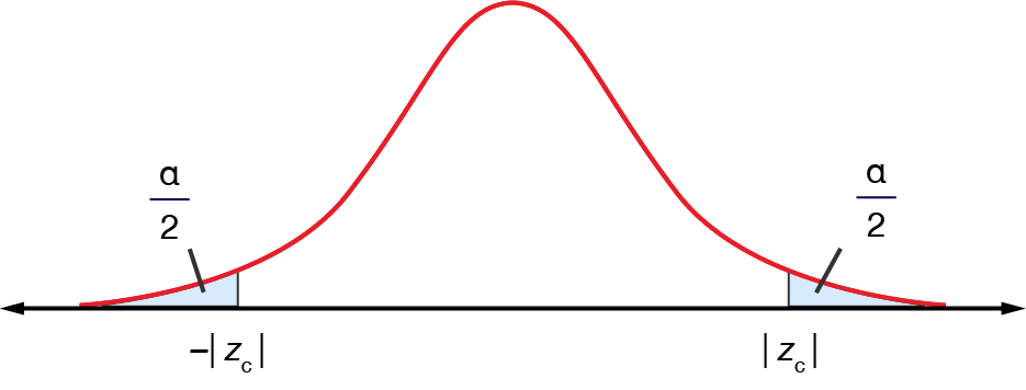
Choose a significance level. Often, we choose \(\alpha=0.05\). In other words, we define "reasonable" as what we can expect \(95\%\) of the time.
Find the critical values (\(z_{c}\)) that correspond to the chosen significance level. These \(z\)-scores are the cutoff points beyond which we reject the null hypothesis.
Calculate the test statistic. This is the standardised difference between the sample mean (calculated from the data) and the known population mean:
\[z = \frac{\overline{x}-\mu}{\frac{\sigma}{\sqrt{n}}}\]
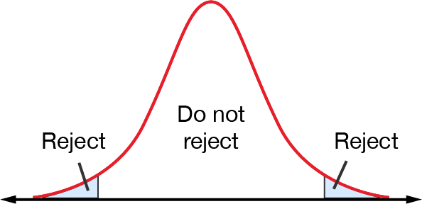
Compare the test statistic to the critical value to make a decision about the null hypothesis.
If the test statistic falls beyond the cutoff point/s of the critical value, we reject the null hypothesis with \(5\%\) confidence, as per the chosen significance level.
If the test statistic falls within the cuttoff point/s of the critical value, we do not reject the null hypothesis with \(5\%\) confidence, as per the chosen significance level.
Draw a conclusion from the hypothesis test.
If we have rejected the null hypothesis, this means that the sample mean is not the same as the population mean after allowing for chance variation.
If we have not rejected the null hypothesis, this means that the sample mean is the same as the population mean after allowing for chance variation.
Remember:
The decision about the null hypothesis is not made with certainty but with a level of confidence that the error in the decision is small; for example, \(5\%\) if \(\alpha=0.05\).
Terminology is important! The decision relates only to rejecting or not rejecting the null hypothesis, \(H_{0}\). We never make a decision that references the alternate hypothesis, \(H_{a}\), nor do we say we "accept" either hypothesis.
This resource outlines just one way of testing a hypothesis. You can read about , and .
Example – conducting \(z\)-tests
Students had previously found a statistics course very difficult, with the average score over many years was \(48\%\) with a standard deviation of \(12\%\). A bridging program was introduced to support students, and in the first year the program ran, the \(120\) students that attended achieved a mean score of\(50\%\) in the final exam. Is there evidence that the scores of those who attended the bridging program have changed, at a \(1\%\) level of significance?
We start with the hypotheses.
\(H_{0}:\overline{x}=48\)
\(H_{a}:\overline{x}\neq48\)
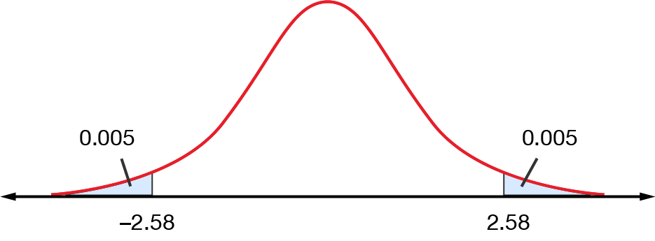
The significance level has been given to us in the question: \(1\%\) means \(\alpha=0.01\).
We use the \(z\)-table to find the critical values. You can go back to Confidence intervals if you need some help finding these.
For \(\alpha=0.01\), \(z=-2.58\) or \(z=2.58\). The interval of interest would be \(\left[-2.58,2.58\right]\).
We use the formula to calculate the test statistic.
\[\begin{align*} z & = \frac{\overline{x}-\mu}{\frac{\sigma}{\sqrt{n}}}\\
& = \frac{50-48}{\frac{12}{\sqrt{120}}}\\
& = 1.83
\end{align*}\]
The test statistic \(1.83\) does not fall outside the cutoffs of \(-2.58\) and \(2.58\), so we do not reject the null hypothesis.
Finally, we can draw a conclusion. Based on the hypothesis test, there is not enough evidence to suggest that the scores of those who attended the bridging program have changed. It is reasonable that the apparent improvement in scores was due to chance variation.
Exercise – conducting \(z\)-tests
Students had previously found a statistics course very difficult, with the average score over many years was \(48\%\) with a standard deviation of \(12\%\). A bridging program was introduced to support students, and in the first year the program ran, the \(120\) students that attended achieved a mean score of\(50\%\) in the final exam. Is there evidence that the scores of those who attended the bridging program have changed, at a \(10\%\) level of significance?
A random sample of \(36\) soft drinks from vending machines had an average content of \(370\textrm{ mL}\) with a standard deviation of \(20\textrm{ mL}\). Test the null hypothesis that \(\mu=375\textrm{ mL}\) against the alternative hypothesis \(\mu\neq375\textrm{ mL}\) at the \(1\%\) significance level.
A bank manager has historical data that shows over lunchtime Mon–Fri, the mean number of customers that come into the bank is \(32\). Accordingly, he believes he has no need to change the number of tellers. However, a branch survey conducted every lunchtime over eight weeks found that the mean number of customers was \(36\) with a standard deviation of \(8.2\).
Conduct a hypothesis test with a \(5\%\) level of significance to test whether the mean number of lunchtime customers has changed.
What recommendation would you make to the bank manager?
The manufacturer of LongLast batteries claims the mean lifetime of his batteries is \(450\) hours. A consumer interest magazine samples \(100\) batteries and finds that they have a mean of \(444\) hours with a standard deviation of \(28\) hours. Does the sample data contradict the manufacturer's claim? Use \(\alpha=0.02\)).
There is enough evidence to suggest that the scores of those who attended the bridging program have changed. We reject the null hypothesis.
There is not enough evidence to suggest that the average content differs from \(375\textrm{ mL}\). We do not reject the null hypothesis.
There is enough evidence to suggest that there is an increase in the number of lunchtime customers. We would recommend that the bank manager increases the number of tellers.
There is not enough evidence to contradict the manufacturer's claim. We do not reject the null hypothesis.