Confidence intervals

When we use the mean of a sample to estimate the mean of an entire population, we use confidence intervals to help us understand the precision of our estimates and how confident we can be about them. This tool is useful for making informed decisions based on sample data. Use this resource to learn how to use confidence intervals.

We use the statistics we obtain from samples to make inferences or estimates about the population from which the sample was drawn.

• A batch may be selected in a factory production process to assess how the process is operating.
• Surveys of consumers are used to determine the preferred brands in the population.
• Polls are conducted on samples of the voting population before elections to predict the result of the election.

But these estimates can vary from one sample to another, so we use tools called confidence intervals. They give us a range of values that likely include the true population parameter, like a mean or proportion.

For example, if we calculate a \(95\%\) confidence interval, it means we expect the true value to fall within that range \(95\%\) of the time if we repeated the experiment many times.

Constructing confidence intervals

Reporting a confidence interval together with our estimate of the population parameter lets us make statements like: "we are \(95\)% confident that the true mean weight of boxes of cereal labelled \(450\textrm{ g}\) is in the interval \([449.5,453.8]\)".

For large samples (\(n\geq30\)), we can use the mean of a sample, \(\overline{x}\), to find an interval estimate for the mean of the population, \(\mu\):

\[\mu=\overline{x}\pm\left(z\times\frac{\sigma}{\sqrt{n}}\right)\]

If the standard deviation for the population data \(\sigma\) is not known, we use the standard deviation for the sample \(s\):

\[\mu=\overline{x}\pm\left(z\times\frac{s}{\sqrt{n}}\right)\]

Probability and confidence intervals

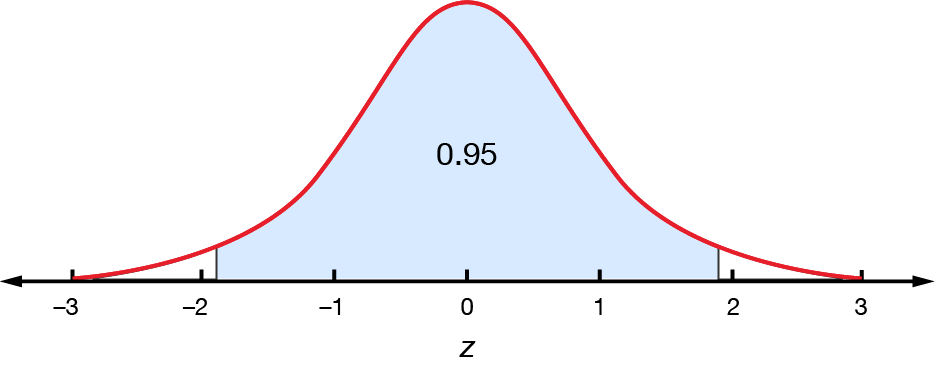
The \(z\)-score is determined by the level of confidence and can be found using \(z\)-tables, a graphics calculator or statistics software.

As shown in the standard normal distribution curve, for a \(95\%\) confidence interval, \(z=1.96\).

Similarly:

• For a \(99\%\) confidence interval, \(z=2.575\).
• For a \(90\%\) confidence interval, \(z=1.645\).

Example – constructing confidence intervals

\(36\) of a certain type of fish were caught in Port Phillip Bay. This sample had a mean length of \(30\textrm{ cm}\) and a standard deviation of \(3\textrm{ cm}\).

1. Constuct a \(95\%\) confidence interval for the true mean length of this type of fish.
2. Construct a \(98\%\) confidence interval for the true mean length of this type of fish.

For the \(95\%\) confidence interval, \(z=1.96\). We only have the standard deviation for the sample, \(s=3\). We substitute these, along with \(\overline{x}=30\) and \(n=36\), into the equation to estimate the mean of the population.
\[\begin{align*} \mu & = \overline{x}\pm\left(z\times\frac{s}{\sqrt{n}}\right)\\
& = 30\pm\left(1.96\times\frac{3}{\sqrt{36}}\right)\\
& = 30\pm0.98\\
& = \left[29.02,30.98\right]
\end{align*}\]

We can state with \(95\%\) confidence that the mean of the entire population of fish will be between \(29.02\textrm{ cm}\) and \(30.98\textrm{ cm}\).

We can do the same for the \(98\%\) confidence. Looking this up on a \(z\)-table, we find that \(z=2.326\).
\[\begin{align*} \mu & = \overline{x}\pm\left(z\times\frac{s}{\sqrt{n}}\right)\\
& = 30\pm\left(2.326\times\frac{3}{\sqrt{36}}\right)\\
& = 30\pm1.163\\
& = \left[28.84,31.16\right]
\end{align*}\]

We can state with \(98\%\) confidence that the mean of the entire population of fish will be between \(28.84\textrm{ cm}\) and \(31.16\textrm{ cm}\).

Exercise – constructing confidence intervals

1. In an effort to improve appointment scheduling, a doctor agreed to estimate the average time spent with each patient. A random sample of \(49\) patients had a mean of \(30\) minutes and a standard deviation of \(7\) minutes.
1. Construct a \(95\%\) confidence interval for the true mean.
2. Construct an \(80\%\) confidence interval for the true mean.
2. To estimate the average weight of males in the town of Cityville, a random sample of \(100\) men was drawn from the population of \(10000\) men and weights were recorded. The mean weight was found to be \(83\textrm{ kg}\) and the standard deviation \(12\textrm{ kg}\).
1. Construct a \(99\%\) confidence interval for the mean weight of the male population.
2. In two of the suburbs of Cityville, Subtown and Tubtown, the mean weights for males were found to be \(80\textrm{ kg}\) and \(88\textrm{ kg}\), repectively. Comment on these results.
3. A market research company conducted a randomised survey of \(50\) regular smokers to find the amount spent on cigarettes per week. They found that the smokers spent on average \(\$22\) each week and the standard deviation was \(\$4.50\). Construct a \(95\%\) confidence interval for the true mean amount spent on cigarettes by regular smokers.
4. After randomly sampling \(400\) individuals and obtaining a sample mean of \(56.5\), a research company was able to claim they were \(90\%\) certain that the true mean of the population was between \(56.089\) and \(56.911\). What was the standard deviation of the sample?