Sampling distributions

Sampling distributions help us understand the behaviour of sample statistics, like means or proportions, from different samples of the same population. By examining these distributions, we can see how sample results might vary and how close they are likely to be to the actual population value. This concept is important for making predictions and decisions based on sample data, such as estimating averages or testing hypotheses.

A sampling distribution is the probability distribution for the means of all samples of size \(n\) from a specific, given population. It gives us an idea of the range of possible statistical outcomes for a population.

Population parameters

There are two key parameters that we look at when we deal with sampling distributions and population data.

• The mean of the sampling distribution, or the mean of all the sample means, is denoted by \(\mu_{\overline{x}}\):
  

  \[\mu_{\overline{x}}=\mu\]

  where \(\mu\) is the population mean.

• The standard deviation of the sampling distribution is denoted by \(\sigma_{\overline{x}}\):
  

  \[\sigma_{\overline{x}}=\dfrac{\sigma}{\sqrt{n}}\]

  where \(\sigma\) is the population standard deviation and \(n\) is the sample size.

The sampling distribution with parameters \(\mu_{\overline{x}}\) and \(\sigma_{\overline{x}}\) tends to follow a normal distribution, if either:

1. the population from which the samples are drawn is normally distributed; or
2. the samples are large \((n\geq30)\).

Properties of a sampling distribution

• The sampling distribution has the same centre as the population.
• \(\sigma_{\overline{x}}\) is the measure of variability of a sampling distribution or the standard error.
• The distribution of means is not as spread out as the values in the population from which the sample was drawn.
• If we do not know the population standard deviation, we approximate with the sample standard deviation: \(s_{\overline{x}}\approx\sigma_{\overline{x}}\) and \(\dfrac{s}{\sqrt{n}}\approx\dfrac{\sigma}{\sqrt{n}}\) if the sample is large.

Probability and sampling distributions

When sampling distributions follow a normal distribution, we can find probabilities (\(\Pr(\overline{X})\)). See Probability and the normal distribution if you need a refresher.

Let's consider the small population of values \(P=1\,2\,3\,4\,5\). This population has \(\mu=3\) and \(\sigma=1.41\). If a sample of size \(n=3\) was drawn from this population, it could be any one of:
\[\begin{array}{cccc} (1\,2\,3) & (1\,2\,4) & (1\,2\,5) & (1\,3\,4)\\
(1\,3\,5) & (1\,4\,5) & (2\,3\,4) & (2\,3\,5)\\
(2\,4\,5) & (3\,4\,5)
\end{array}\]

The means of each of the samples are shown in the table.

Sample	Mean
\((1\,2\,3)\)	\(\overline{x}=2\)
\((1\,2\,4)\)	\(\overline{x}=2.33\)
\((1\,2\,5)\)	\(\overline{x}=2.67\)
\((1\,3\,4)\)	\(\overline{x}=2.67\)
\((1\,3\,5)\)	\(\overline{x}=3\)
\((1\,4\,5)\)	\(\overline{x}=3.33\)
\((2\,3\,4)\)	\(\overline{x}=3\)
\((2\,3\,5)\)	\(\overline{x}=3.33\)
\((2\,4\,5)\)	\(\overline{x}=3.67\)
\((3\,4\,5)\)	\(\overline{x}=4\)

From this, we can calculate the population mean and standard deviation:
\[\begin{align*} \mu_{\overline{x}} & = \frac{\sum \overline{x}_{n}}{n}\\
& = \frac{30}{10}\\
& = 3
\end{align*}\] \[\begin{align*} \sigma_{\overline{x}} & = \frac{\sigma}{\sqrt{n}}\\
& = \sqrt {\frac {\sum (x-\overline{x})^{2} } {n-1} } \times \frac{1}{\sqrt{n}}\\
& = \frac{1.92}{\sqrt{10}}\\
& = 0.61
\end{align*}\]

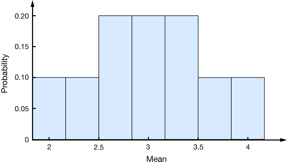
By converting the values to \(z\)-scores, we can find the probabilities where \(\Pr(\overline{X}=\overline{x})\), as shown in the table.

\(\mathbf{\overline{x}}\)	\(2\)	\(2.33\)	\(2.67\)	\(3\)	\(3.33\)	\(3.67\)	\(4\)
\(\mathbf{\Pr(\overline{X}=\overline{x}}\))	\(0.1\)	\(0.1\)	\(0.2\)	\(0.2\)	\(0.2\)	\(0.1\)	\(0.1\)

Plotting the distribution of means on a histogram, we can see that even though the sample is small and the population is not normally distributed (though it is symmetric), the sampling distribution is reasonably normally distributed.

Here, the mean of the sampling distribution (the mean of all the means) is the same as the population mean, \(\mu_{\overline{x}}=\mu=3\).

However, the variability in the sampling distribution is less than that of the population: \(\sigma_{\overline{x}}=0.61\) and \(\sigma=1.41\).

Larger samples, or those drawn from normally distributed populations will follow a normal distribution, so we can use the properties of normal distributions to find probabilities relating to samples:

\[\begin{align*} z_{\overline{x}} & = \frac{\overline{x}-\mu}{\sigma_{\overline{x}}}\\
& = \frac{\overline{x}-\mu}{\frac{\sigma}{\sqrt{n}}}
\end{align*}\]

Example – calculating probabilities for sampling distributions

The shire of Bondara has \(1200\) preschoolers. The mean weight of preschoolers is known to be \(18\textrm{ kg}\) with a standard deviation of \(3\textrm{ kg}\). What is the probability that a random sample of \(50\) preschoolers will have a mean weight more than \(19\textrm{ kg}\)?

Here, \(n=50\), \(\mu=18\) and \(\sigma=3\). We are looking for \(\Pr(\overline{X}>19)\).

The sampling distribution of the means for samples of size \(50\) will have \(\mu_{\overline{x}}=\mu=18\) and standard error:
\[\begin{align*} \sigma_{\overline{x}} & = \frac{\sigma}{\sqrt{n}}\\
& = \frac{3}{\sqrt{50}}\\
& = 0.42
\end{align*}\]

From this, we can convert the value of interest into a \(z\)-score, which we can then look up on a \(z\)-table.
\[\begin{align*} z_{\overline{x}} & = \frac{\overline{x}-\mu}{\frac{\sigma}{\sqrt{n}}}\\
& = \frac{19-18}{\frac{3}{\sqrt{50}}}\\
& = 2.38
\end{align*}\]

Finally, we can calculate the probability.
\[\begin{align*} \Pr(\overline{x}>19) & = \Pr(z_{\overline{x}}>2.38)\\
& = 1-0.9913\\
& = 0.0087
\end{align*}\]

Exercise – calculating probabilities for sampling distributions

1. List all samples of size \(2\) for the population \((1\,2\,3\,4\,5\,6)\), then find the probability of obtaining a sample mean of less than \(3\).
2. Samples of size \(40\) are drawn from a population with \(\mu=50\) and \(\sigma=5\).
   1. What are the mean and standard error of the sampling distribution?
   2. What is the probability that a particular sample has a mean less than \(48.5\)?
3. If IQ in the general population of secondary students is known to follow a normal distribution with \(\mu=100\) and \(\sigma=10\):
   1. Find the mean and standard error for a random sample of size \(100\).
   2. To test whether a secondary school is representative of the general population, a sample of \(100\) students from that school is chosen. What is the probability of the mean IQ being more than \(105\)? What would be your conclusion?